3D Gaussian Splatting for Real-Time Radiance Field Rendering

This repository contains the official authors implementation associated with the paper "3D Gaussian Splatting for Real-Time Radiance Field Rendering", which can be found here. We further provide the reference images used to create the error metrics reported in the paper, as well as recently created, pre-trained models.

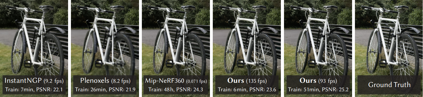
Abstract: Radiance Field methods have recently revolutionized novel-view synthesis of scenes captured with multiple photos or videos. However, achieving high visual quality still requires neural networks that are costly to train and render, while recent faster methods inevitably trade off speed for quality. For unbounded and complete scenes (rather than isolated objects) and 1080p resolution rendering, no current method can achieve real-time display rates. We introduce three key elements that allow us to achieve state-of-the-art visual quality while maintaining competitive training times and importantly allow high-quality real-time (≥ 30 fps) novel-view synthesis at 1080p resolution. First, starting from sparse points produced during camera calibration, we represent the scene with 3D Gaussians that preserve desirable properties of continuous volumetric radiance fields for scene optimization while avoiding unnecessary computation in empty space; Second, we perform interleaved optimization/density control of the 3D Gaussians, notably optimizing anisotropic covariance to achieve an accurate representation of the scene; Third, we develop a fast visibility-aware rendering algorithm that supports anisotropic splatting and both accelerates training and allows realtime rendering. We demonstrate state-of-the-art visual quality and real-time rendering on several established datasets.

@Article{kerbl3Dgaussians,
      author       = {Kerbl, Bernhard and Kopanas, Georgios and Leimk{\"u}hler, Thomas and Drettakis, George},
      title        = {3D Gaussian Splatting for Real-Time Radiance Field Rendering},
      journal      = {ACM Transactions on Graphics},
      number       = {4},
      volume       = {42},
      month        = {July},
      year         = {2023},
      url          = {https://repo-sam.inria.fr/fungraph/3d-gaussian-splatting/}
}

Funding and Acknowledgments

This research was funded by the ERC Advanced grant FUNGRAPH No 788065. The authors are grateful to Adobe for generous donations, the OPAL infrastructure from Université Côte d’Azur and for the HPC resources from GENCI–IDRIS (Grant 2022-AD011013409). The authors thank the anonymous reviewers for their valuable feedback, P. Hedman and A. Tewari for proofreading earlier drafts also T. Müller, A. Yu and S. Fridovich-Keil for helping with the comparisons.

NEW FEATURES !

We have limited resources for maintaining and updating the code. However, we have added a few new features since the original release that are inspired by some of the excellent work many other researchers have been doing on 3DGS. We will be adding other features within the ability of our resources.

Update of October 2024: We integrated training speed acceleration and made it compatible with depth regularization, anti-aliasing and exposure compensation. We have enhanced the SIBR real time viewer by correcting bugs and adding features in the Top View that allows visualization of input and user cameras.

Update of Spring 2024: Orange Labs has kindly added OpenXR support for VR viewing.

Step-by-step Tutorial

Jonathan Stephens made a fantastic step-by-step tutorial for setting up Gaussian Splatting on your machine, along with instructions for creating usable datasets from videos. If the instructions below are too dry for you, go ahead and check it out here.

Colab

User camenduru was kind enough to provide a Colab template that uses this repo's source (status: August 2023!) for quick and easy access to the method. Please check it out here.

Cloning the Repository

The repository contains submodules, thus please check it out with

# SSH
git clone [email protected]:graphdeco-inria/gaussian-splatting.git --recursive

# HTTPS
git clone https://github.com/graphdeco-inria/gaussian-splatting --recursive

Overview

The codebase has 4 main components:

• A PyTorch-based optimizer to produce a 3D Gaussian model from SfM inputs
• A network viewer that allows to connect to and visualize the optimization process
• An OpenGL-based real-time viewer to render trained models in real-time.
• A script to help you turn your own images into optimization-ready SfM data sets

Optimizer

The optimizer uses PyTorch and CUDA extensions in a Python environment to produce trained models.

Hardware Requirements

• CUDA-ready GPU with Compute Capability 7.0+
• 24 GB VRAM (to train to paper evaluation quality)
• Please see FAQ for smaller VRAM configurations

Software Requirements

• Conda (recommended for easy setup)
• C++ Compiler for PyTorch extensions (we used Visual Studio 2019 for Windows)
• CUDA SDK 11 for PyTorch extensions, install after Visual Studio (we used 11.8, known issues with 11.6)
• C++ Compiler and CUDA SDK must be compatible

Setup

Local Setup

Our default, provided install method is based on Conda package and environment management:

SET DISTUTILS_USE_SDK=1 # Windows only
conda env create --file environment.yml
conda activate gaussian_splatting

Tip: Downloading packages and creating a new environment with Conda can require a significant amount of disk space. By default, Conda will use the main system hard drive. You can avoid this by specifying a different package download location and an environment on a different drive:

conda config --add pkgs_dirs /<pkg_path>
conda env create --file environment.yml --prefix /<env_path>/gaussian_splatting
conda activate /<env_path>/gaussian_splatting

Modifications

If you can afford the disk space, we recommend using our environment files for setting up a training environment identical to ours. If you want to make modifications, please note that major version changes might affect the results of our method. However, our (limited) experiments suggest that the codebase works just fine inside a more up-to-date environment (Python 3.8, PyTorch 2.0.0, CUDA 12). Make sure to create an environment where PyTorch and its CUDA runtime version match and the installed CUDA SDK has no major version difference with PyTorch's CUDA version.

Known Issues

Some users experience problems building the submodules on Windows (``cl.exe: File not found`` or similar). Please consider the workaround for this problem from the FAQ.

Running

To run the optimizer, simply use

python train.py -s 

Note that similar to MipNeRF360, we target images at resolutions in the 1-1.6K pixel range. For convenience, arbitrary-size inputs can be passed and will be automatically resized if their width exceeds 1600 pixels. We recommend to keep this behavior, but you may force training to use your higher-resolution images by setting ``-r 1``.

The MipNeRF360 scenes are hosted by the paper authors here. You can find our SfM data sets for Tanks&Temples and Deep Blending here. If you do not provide an output model directory (``-m`), trained models are written to folders with randomized unique names inside the `output`` directory. At this point, the trained models may be viewed with the real-time viewer (see further below).

Evaluation

python train.py -s  --eval # Train with train/test split
python render.py -m  # Generate renderings
python metrics.py -m  # Compute error metrics on renderings

If you want to evaluate our pre-trained models, you will have to download the corresponding source data sets and indicate their location to ``render.py` with an additional `--source_path/-s`` flag. Note: The pre-trained models were created with the release codebase. This code base has been cleaned up and includes bugfixes, hence the metrics you get from evaluating them will differ from those in the paper.

python render.py -m  -s 
python metrics.py -m 

We further provide the ``full_eval.py` script. This script specifies the routine used in our evaluation and demonstrates the use of some additional parameters, e.g., `--images (-i)`` to define alternative image directories within COLMAP data sets. If you have downloaded and extracted all the training data, you can run it like this:

python full_eval.py -m360  -tat  -db 

python full_eval.py -o  --skip_training -m360  -tat  -db 

If you want to compute the metrics on our paper's evaluation images, you can also skip rendering. In this case it is not necessary to provide the source datasets. You can compute metrics for multiple image sets at a time.

python full_eval.py -m /garden ... --skip_training --skip_rendering

Interactive Viewers

Hardware Requirements

• OpenGL 4.5-ready GPU and drivers (or latest MESA software)
• 4 GB VRAM recommended
• CUDA-ready GPU with Compute Capability 7.0+ (only for Real-Time Viewer)

Software Requirements

• Visual Studio or g++, not Clang (we used Visual Studio 2019 for Windows)
• CUDA SDK 11, install after Visual Studio (we used 11.8)
• CMake (recent version, we used 3.24)
• 7zip (only on Windows)

Pre-built Windows Binaries

Installation from Source

Windows

cd SIBR_viewers
cmake -Bbuild .
cmake --build build --target install --config RelWithDebInfo

Ubuntu 22.04

# Dependencies
sudo apt install -y libglew-dev libassimp-dev libboost-all-dev libgtk-3-dev libopencv-dev libglfw3-dev libavdevice-dev libavcodec-dev libeigen3-dev libxxf86vm-dev libembree-dev
Project setup
cd SIBR_viewers
cmake -Bbuild . -DCMAKE_BUILD_TYPE=Release # add -G Ninja to build faster
cmake --build build -j24 --target install

Ubuntu 20.04

git checkout fossa_compatibility

Navigation in SIBR Viewers

Running the Network Viewer

https://github.com/graphdeco-inria/gaussian-splatting/assets/40643808/90a2e4d3-cf2e-4633-b35f-bfe284e28ff7

After extracting or installing the viewers, you may run the compiled ``SIBR_remoteGaussian_app[_config]` app in `/bin``, e.g.:

.//bin/SIBR_remoteGaussian_app

Running the Real-Time Viewer

https://github.com/graphdeco-inria/gaussian-splatting/assets/40643808/094